Last Updated: March 7, 2023

Well after over four weeks of work, I finally have the withdrawal method stress testing results of the Tax and Penalty Minimization (TPM) withdrawal method and the Traditional withdrawal method! Woohoo! Not just another “update” post!
I hope you’re psychologically prepared for plots. LOTS of plots. But really, who doesn’t love plots? They’re the best.
Before we dive into the analysis done and the results generated, first some thoughts on dividend yields and a bug fix.
Dividend Yield
Last week I discussed how I’m now using the published multi-year average dividend yields for relevant low cost index funds, to come up with a reasonable amount of dividends received each year from the post-tax account (yield * account balance = dividend amount).
Before I tried stressing this method, I didn’t even think about using a non-constant dividend amount. That was a major “duh” moment for me, especially when I saw dividends coming in with a $0 account balance!
Initially I thought this simple multiplication of the overall asset balance wasn’t the greatest model, because dividends are computed as a function of how many shares you have. But it would be a significant amount of work to do something higher fidelity, so put that on my future task list.
But the more I thought about it, the more convinced I became that this approach is likely more solid than I initially expected.
Dividend yields are pretty stable actually, and near historic lows. Looking at dividend yields for VTSAX and VHYAX for the last 3 to 5 years, they’re typically within 0.5% of the multi-year average.
Why are yields so stable though?
A) The number of companies in those funds is large enough to significantly reduce volatility.
B) Equity prices are in the denominator of the yield calculation. If we have a bear market with a 20% drop in equity prices, that will increase the dividend yield by 25% – but that increases a dividend yield of 1.5% to just 1.875%.
So as long as you pick a dividend yield that is reasonably conservative (i.e. no higher than the 5 year average, and perhaps closer to the 5 year minimum), I think it’s reasonable to take this approach when running the simulation.

Bug Fix – Roth Contributions/Conversions
Something else this stress testing uncovered is a bug lurking in the Roth withdrawal code.
I track both Roth original contributions and conversions to determine if and when those funds can be withdrawn without penalty if you’re under 60. Pretty straightforward.
But, previously I didn’t account for a NEGATIVE ROI (see “Varying ROI” analysis below). Which meant that the Roth balance could easily shrink BELOW the original contributions and/or conversions.
So now any time in the code (TPM or Traditional method) it attempts to withdraw from a Roth account, I determine which value is smaller (contribution/conversion or the account balance), and I use that smaller value for the withdrawal.
That also means that you can draw down your Roth balance to $0, and still have a non-zero contributions / conversion amount! But that’s OK, because the code will always use the minimum for the withdrawal, which is $0 in that scenario.
Varying Expenses
First up – varying expenses. How do both methods fare for a wide range of expenses, from less than expected to much more than expected?
And there are two possible final metrics to track for each expense level – final asset balance (if the sim doesn’t run out of money) or the age that money runs out.
We’ll focus on a lower range of expenses levels ($30K to $80K) for looking at final asset balances (since higher expense levels just give the same $0 final value for the entire span), and a higher range ($60K to $120K) when looking at “Out of Money Age” (since lower levels don’t run out of money).
Betty’s Filing Status: Single
As usual, we’re employing Betty for the single filer example. Apparently Betty fell out of the top 1000 girl names after 1996 – it’s time for a comeback!
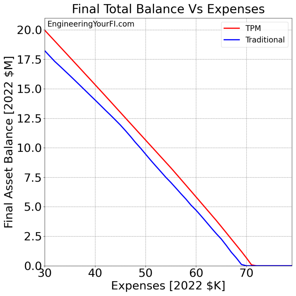
Let’s kick things off by looking at Betty’s final total balance over the 52 year simulation for annual expenses (in 2022 dollars) ranging from $30K to $80K, for both the TPM and Traditional methods:
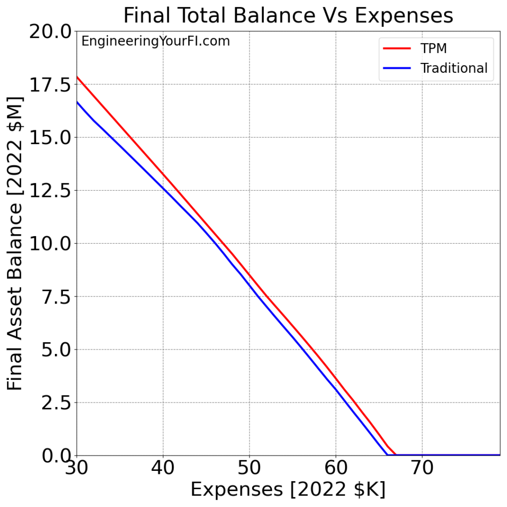
When I first saw this plot, I was amazed how linear the results were. I expected a more exponential plot, but it’s actually a pretty straight downward slope until it slams into $0 shortly before $70K.
Also pretty incredible is how wealthy Betty will be (assuming the historical average annual 7% after-inflation market return) at age 92 if she can stay within $10K of her original $40K expense level (i.e. following the 4% rule for her $1M portfolio).
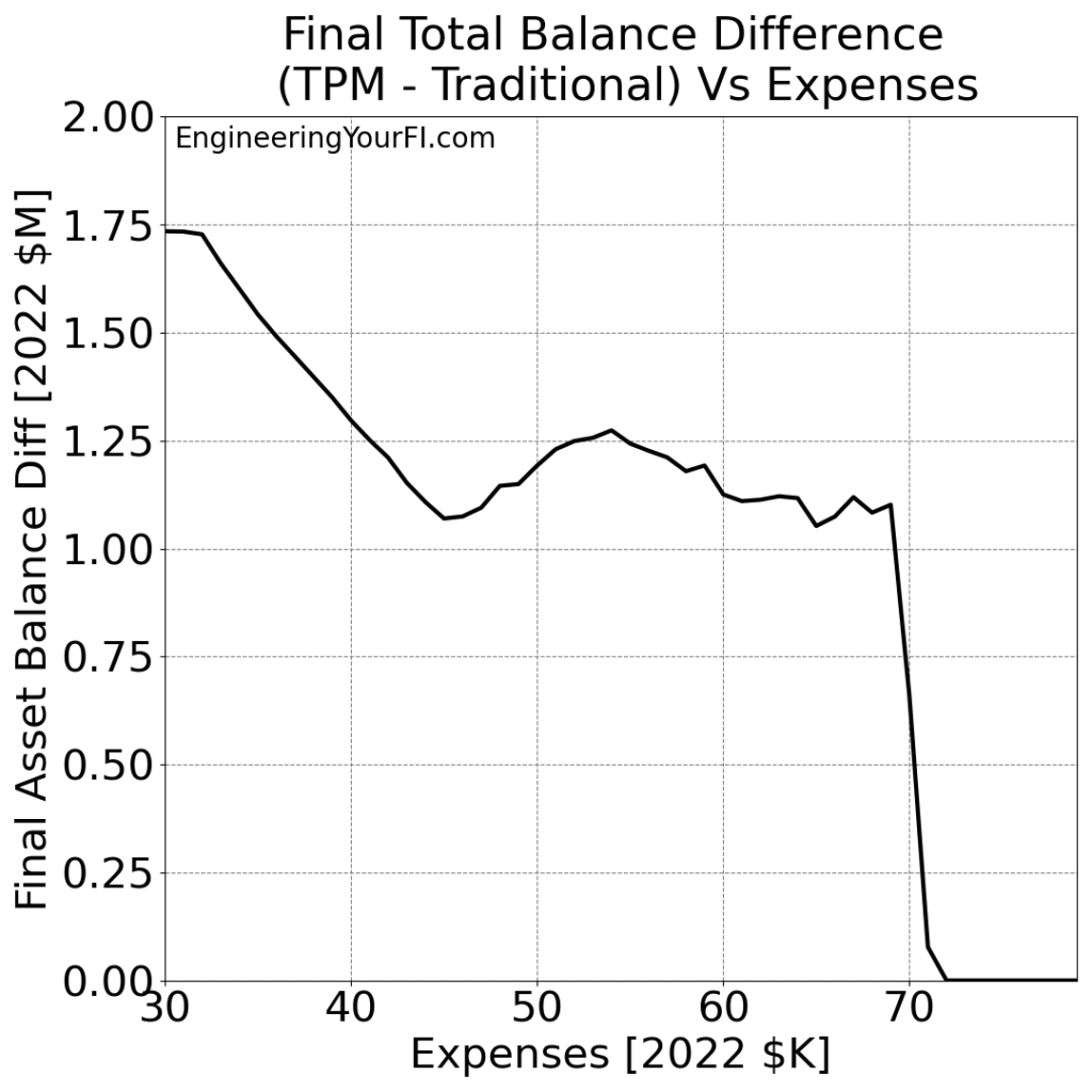
Also very interesting is how the TPM method consistently beats the pants off the Traditional method. Let’s plot the TPM minus Traditional difference in the final asset values:
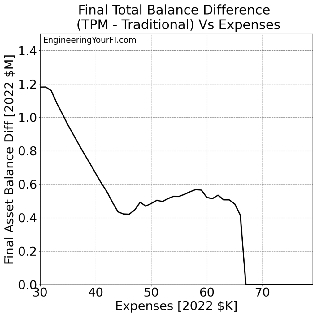
So unlike the previous plot, this doesn’t appear linear at all! It starts pretty high (over a million dollars higher), then shrinks down to a quasi-plateau that slightly drifts down, before money runs out for both methods shortly before $70K.
We can discern a trend though: with smaller expenses, the TPM method does even better relative to the traditional method, and that performance gap shrinks with higher expenses.
Which makes sense to me – as the expenses get more aggressive, I would expect the advantages of the TPM method to shrink.
But most importantly, the TPM method never does WORSE than the traditional method. So you don’t have to decide which one works better for a particular expense level – just always use TPM!
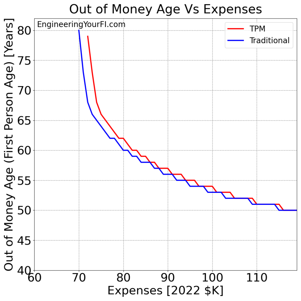
Next up, let’s look at a higher range of expenses and plot when each method runs out of money:
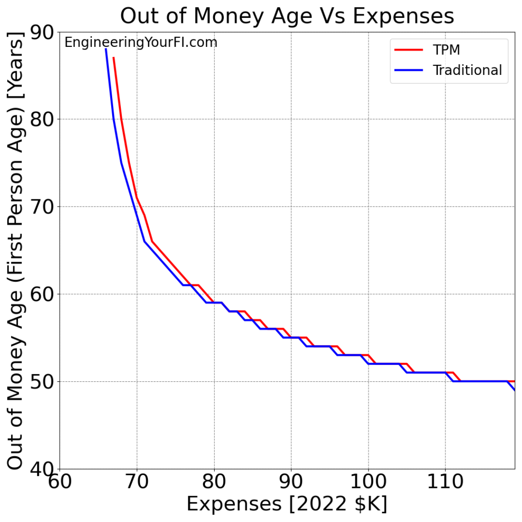
As we saw in the previous two plots, Betty runs out of money before age 92 with expenses around $70K or higher. The traditional method first runs out of expenses at $66K, and the TPM method at $67K.
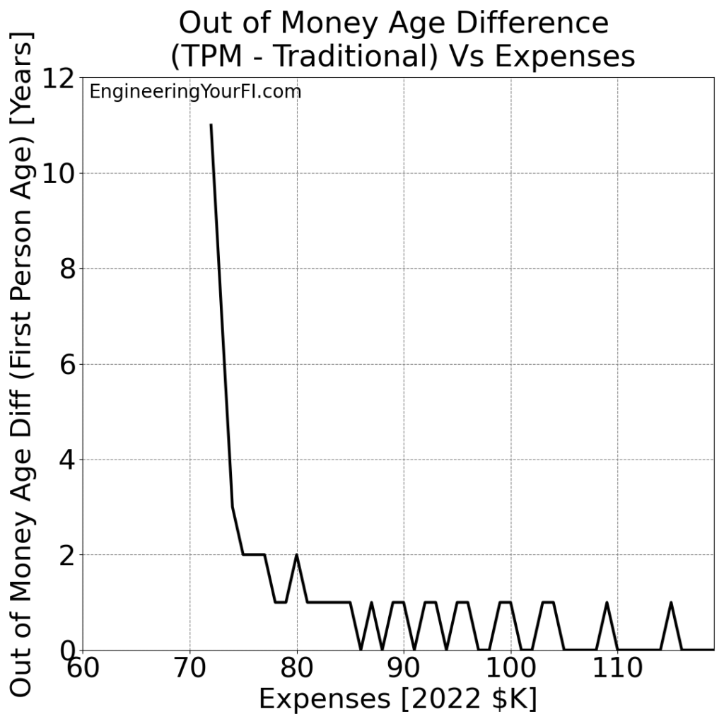
Looking at the difference in Out of Money Ages in a new plot:
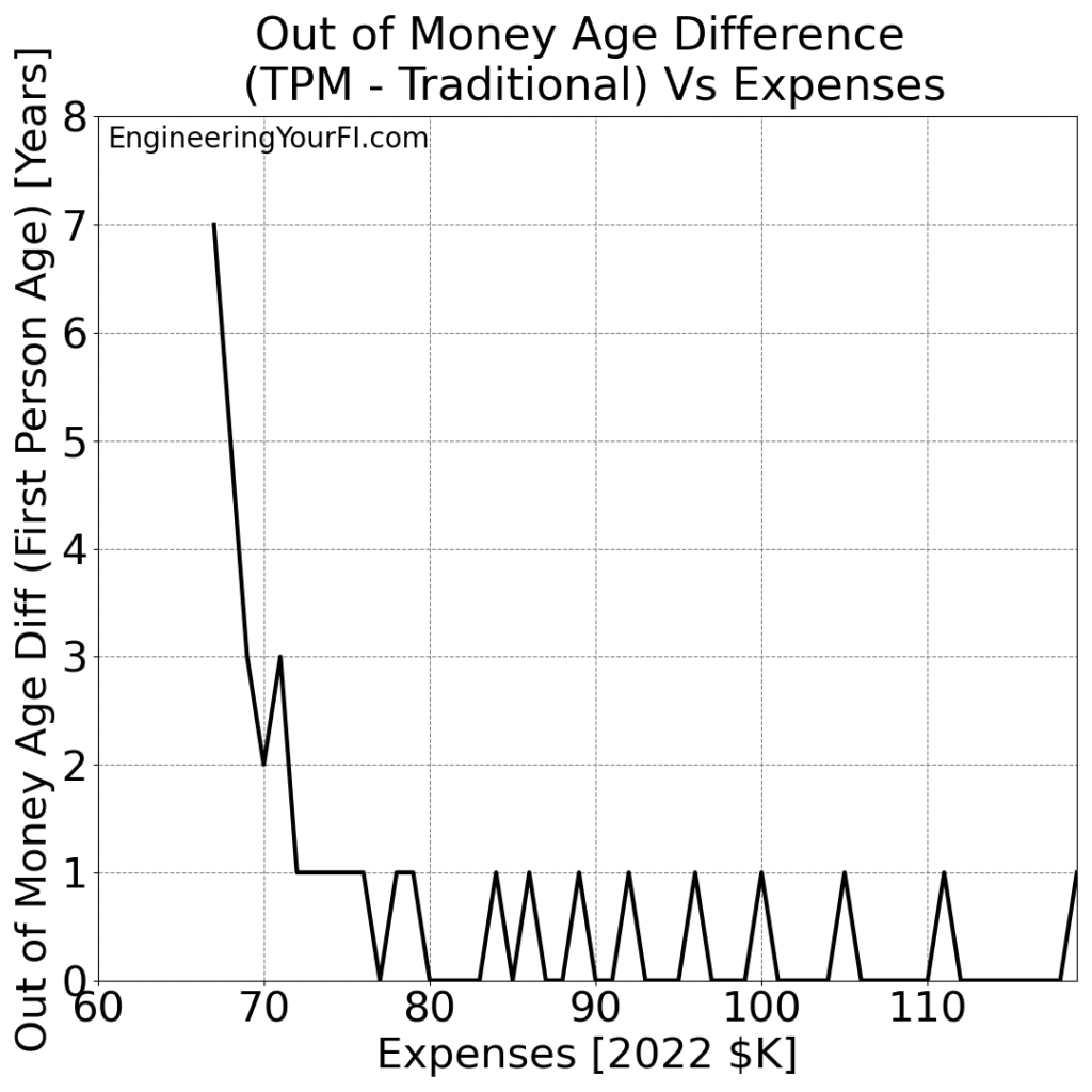
Around $70K, the TPM method buys you quite a few more years vs the traditional method – up to 7 more years at $67K! But around $75K, the difference drops to a year or less.
Just like for final asset values, the two methods seem to converge with increasingly large expense levels, as the advantages of the TPM shrink.
And again, just like for final asset values, the TPM method NEVER does worse than the traditional method. TPM always runs out of money at the same or a later age than the traditional method. So always go with TPM.

Bill and Barbara’s Filing Status: Married Filing Jointly
Just like Betty is proving to be our ultimate repeat “single filer” guest, the married couple Bill and Barbara keep returning as our repeat “married filing jointly” guests.
Bill is in the same boat as Betty, falling out of the top 1000 boy names after 1993, but Barbara is just barely hanging in there as #911 most popular girl name in 2021!
But I’m sure after this article is published, all these names will rocket to the top of charts – I mean who wouldn’t want to be the star of retirement withdrawal analysis?
Now, back to the analysis! Remember all the plots we made for Betty above? Well, we’re just going to repeat those same plots for Bill and Barbara. And great news: all the conclusions are identical.
Bill and Barbara’s final total balance over the 52 year simulation for annual expenses (in 2022 dollars) ranging from $30K to $80K, for both the TPM and Traditional methods:
The TPM minus Traditional difference in the final asset values:
Looking at a higher range of expenses and plotting the “Out of Money Age” for both methods:
Finally, the difference in “Out of Money Ages” between the two methods:
The same conclusions hold for Bill and Barbara as we gathered for Betty: the TPM method always does the same or better versus the Traditional method, but for higher expenses the advantages of the TPM method shrink and thus the performance of the two methods converges.

Varying ROI
Next up: varying the average annual after-inflation market return (Return On Investment, ROI) that we use for every year of the 52 year simulation. While the historical average is 7%, I really wanted to see how sensitive both methods were to changes in this value.
E.g. what if the markets don’t do as well in the next 52 years as the last 52 years?
Of course I recognize that by using the historical average for each year, we are not at all capturing the sequence of returns risk (i.e. if the markets do worse than average early in your retirement).
But NO ONE knows what the future holds, so I’m content with using a single average long term ROI for my analysis (at least for now). And I believe that’s also a reasonable assumption when trying to compare two different withdrawal methods (TPM vs Traditional).
So, let’s vary that single average long term ROI from -7% to +14%, and see how each method does.
And just like for the Expense variation analysis above, we’ll track two main metrics for each ROI value: final asset balance (if the sim doesn’t run out of money) or the age that money runs out.
Betty’s Filing Status: Single
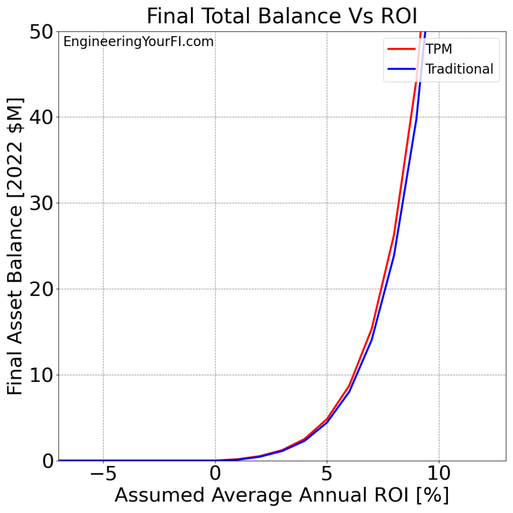
Back to Betty – as always! Let’s look at Betty’s final assets for both methods for the range of ROI values:
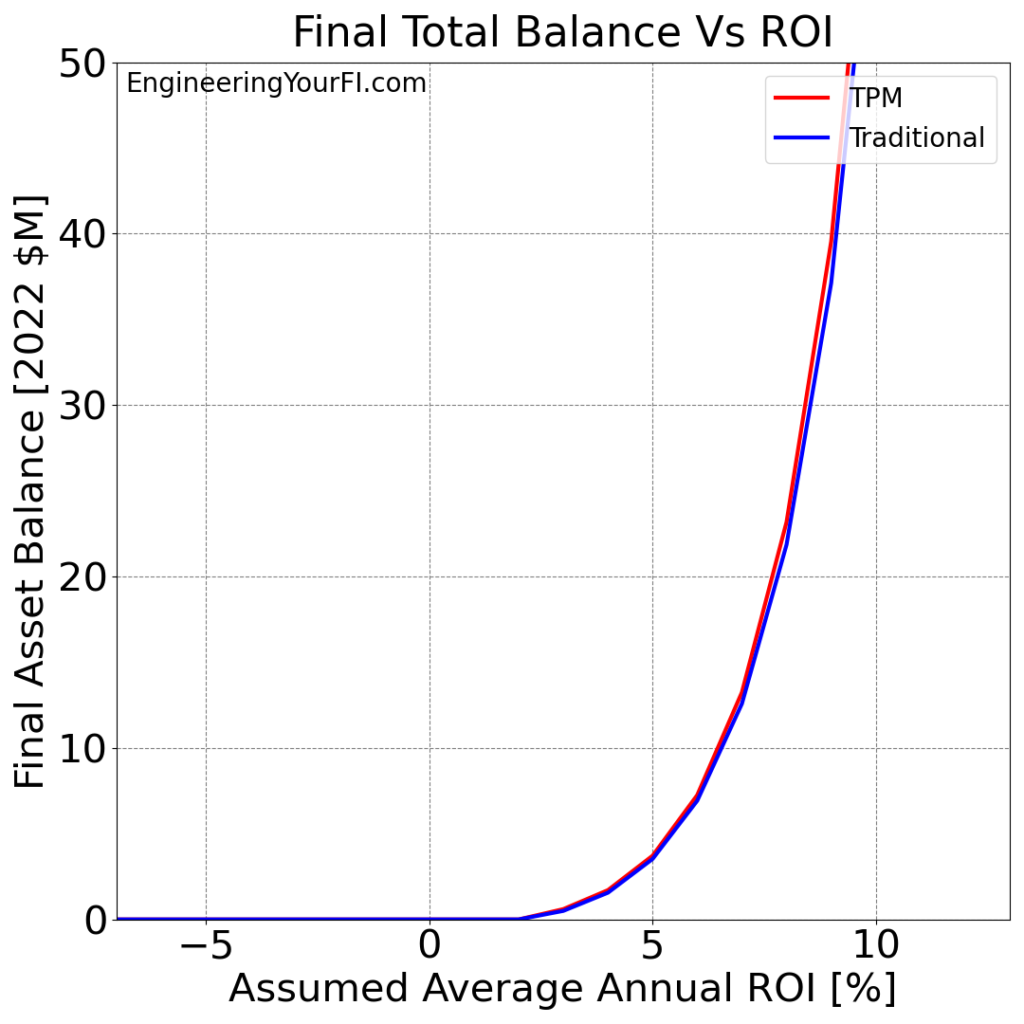
Well unlike the expense variation plots, varying the ROI definitely gives an exponential plot! Which makes sense.
I cut off the plot at $50M to make the plot easier to discern at lower ROI values, but it climbs into the hundreds of millions of dollars for the ROIs exceeding 10% – the power of compounding!
As the ROI increases, the TPM method really starts to pull away from the traditional method. This result matches my intuition: the impact on your final balance from tax/penalty savings achieved via the TPM method each year is going to be magnified by higher ROIs.
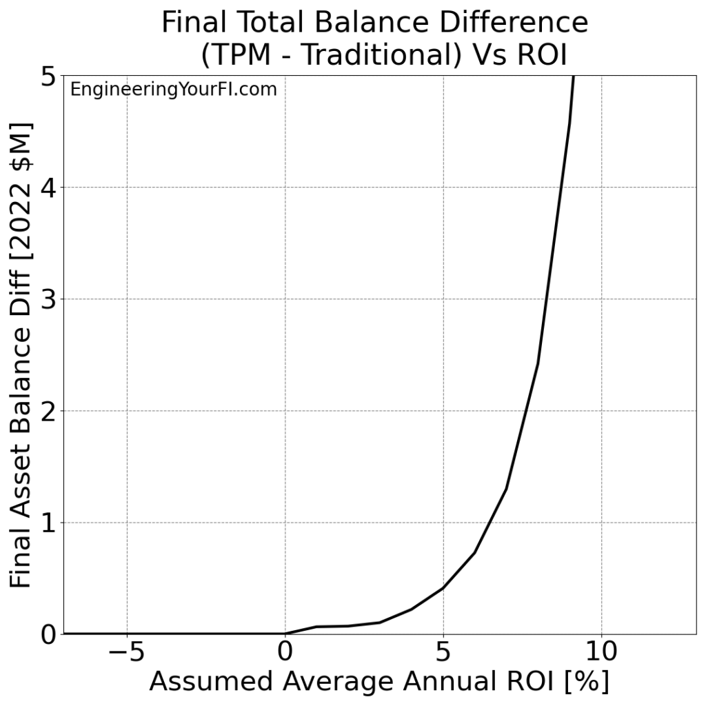
Let’s next plot the difference in the final asset balance for the two methods:
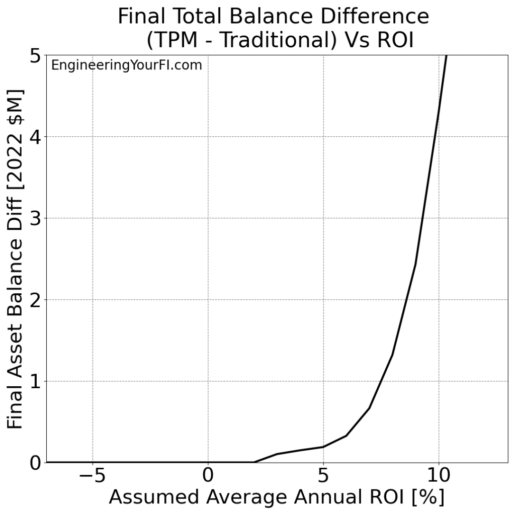
This plot makes it even easier to see how the TPM method results run away from the Traditional method results for higher ROI values. And it also makes it easier to see how Betty won’t run out of money as long as the average ROI is 3% or higher.
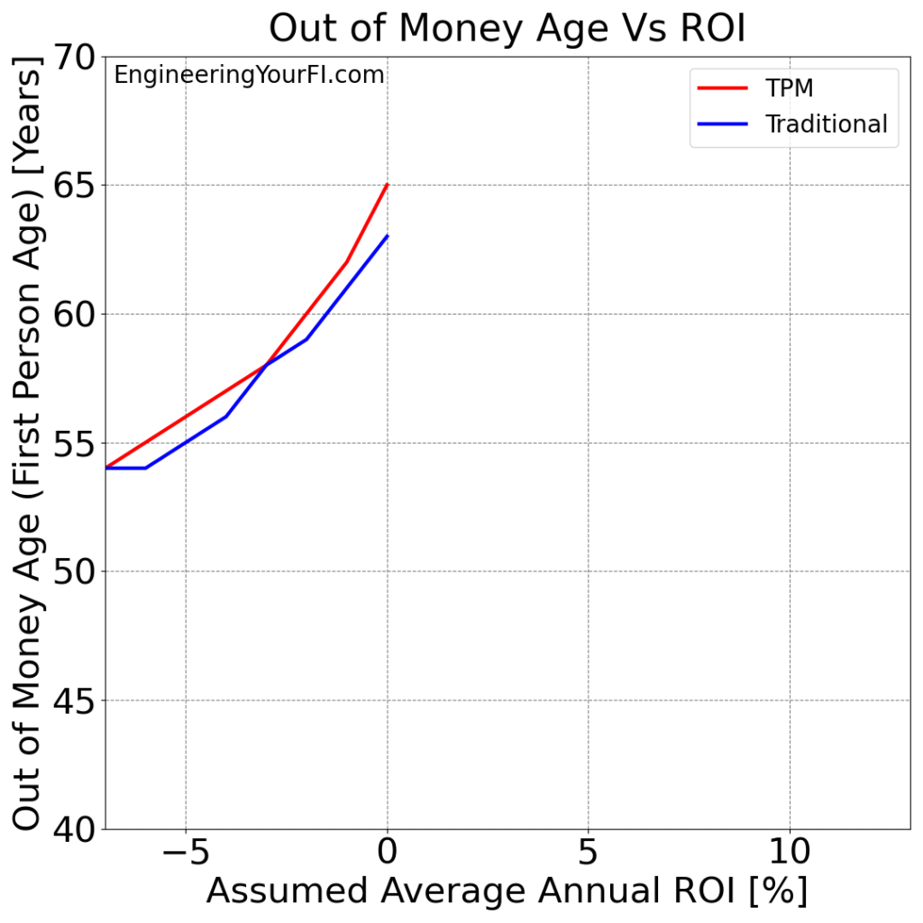
Speaking of running out of money, let’s next plot the “Out of Money Age” for each ROI for each method:
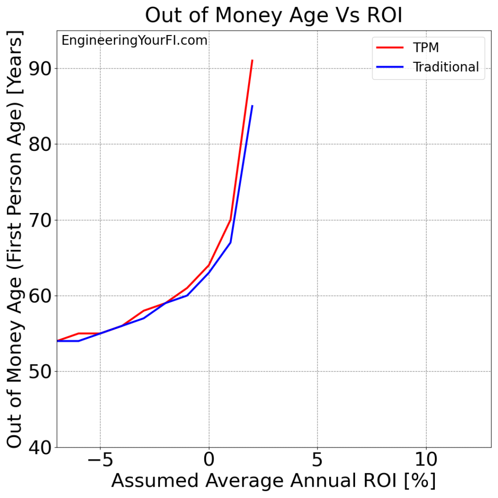
We can see both methods run out of money for ROI values at 2% or lower.
But as usual the TPM always matches or exceeds (sometimes greatly) the Traditional method.
This plot also provides a nice validation of the simulation: if the ROI is 0%, and Betty retires at age 40 with a 4% withdrawal rate (i.e. her assets are 25x her annual expenses), then I would expect her money to last 25 years – when she’s 65 years old. And that’s basically what we see in the plot!
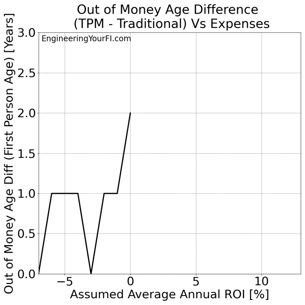
Finally, let’s take a look at the “Out of Money Age” difference for the two methods:
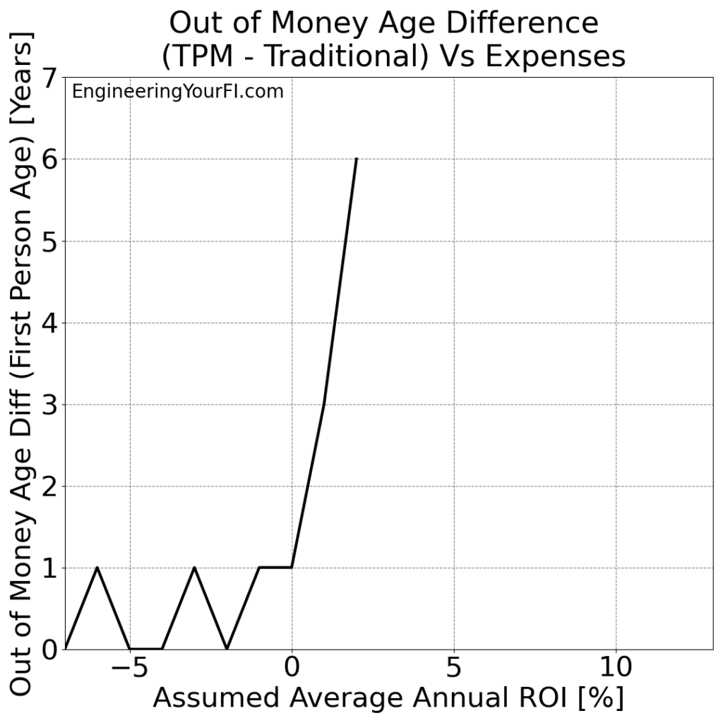
At 2% ROI we see the TPM method buy Betty six additional years, and at 1% ROI the TPM method buys her three extra years, but any ROI less than that doesn’t buy her nearly as much additional time.
Bill and Barbara’s Filing Status: Married Filing Jointly
Just like we keep using Betty for our “single-filer”, we’ll keep using Bill and Barbara as our “married filing jointly” couple.
We’ll show all the same plots for Bill and Barbara that we did for Betty for this ROI variation analysis. And once again, the conclusions are essentially the same.
Bill and Barbara’s final assets for both methods for the range of ROI values:
And the difference in the final asset balance for the two methods:
Bill and Barbara are a bit more fortunate than Betty: as long as the average ROI is 1% or higher, they won’t run out of money.
Also interesting is the plateau in the “TPM Minus Traditional” final asset balance difference from 1% to 3% ROI – off the top of my head, I don’t understand why that’s the case. Why would the TPM advantage over Traditional be the same at 3% ROI as 1% ROI? Something to think about and perhaps investigate further.
Next let’s next plot the “Out of Money Age” for each ROI for each method:
And the difference in “Out of Money Age” for each method:
At 0% ROI we see the TPM method buy Bill and Barbara two additional years, but any ROI less than that gives just one or zero more years.
Code
If you’d like to plug in your own values and play with different withdrawal scenarios to see if you can come out ahead with early withdrawals, you can download the Python code and run it yourself.
In past posts I’ve provided an embedded Python interpreter in this Code section that you can run directly in the browser, but the codebase has now jumped up to 29 files, which makes it a bit unwieldy for a simple embedded interpreter interface. But if you’d really like to have that, let me know and I’ll see if I can make it happen.
Future Work
I am super happy to finally have the above stress testing results. I have long wanted to see how both the TPM and traditional methods do for a range of expense levels (what you control most) and ROI levels (what you control the least).
But, there are other parameters we could do similar sensitivity analysis for:
- Initial asset balances
- Social security payment amount and starting age
- Dividend yield (e.g., if you’ve intentionally invested in funds with higher yields, such as VHYAX instead of VTSAX)
- Future expense changes (e.g., if you decide to pay off some or all of your mortgage, or take on a new mortgage)
Essentially any input parameter the user can specify!
The previous post lists other relevant future work as well. I’m particularly interested in pursuing ideas #1 and #2 in the “Other Ideas” section of that post, which might have a significant impact on the above stress testing results. Fortunately I’m pretty certain that implementing those ideas will only improve the performance of the TPM method relative to the traditional method.
Conclusions
The main conclusion you should take away from all these plots: the TPM method nearly always does better (sometimes MUCH better) than the traditional method for a wide range of expense levels and average market returns. And it NEVER does worse – so there’s no reason (from a performance perspective) to ever choose the traditional method over the TPM method.
The TPM’s improved performance over the Traditional method does shrink with higher expenses and lower market returns though, as the tax and penalty savings have less runway to make a substantial impact.