Last Updated: January 15, 2023

Well after a great deal of work, I have finally extended the Tax and Penalty Minimization (TPM) method to be able to go down to $0! Which I’ve been working on for several weeks.
Unfortunately I ran out of time to do much of any stress testing analysis, but I did run it for a couple scenarios and compared the results to the Traditional method for those scenarios – and the results are very promising!
TPM Numerical Integration
As I mentioned in the previous update post, I decided to use a numerical integration approach to map the path down to $0 in assets. This approach progresses from the lowest taxes and penalties to the largest, so that hopefully your money will last as long as possible. Because trying to find an analytical approach was becoming nightmarishly complicated – I provided a list of the main complications in that same post.
One of the major caveats I mentioned in the previous post was that numerical approaches nearly always require more computing than analytical approaches. So as soon as the numerical integration was in place and I felt comfortable that it was reasonably well tested, I tried four different step values, ranging from $1 to $1000:
- $1: Total Final = $381595.14, Sim Time = 242.99 seconds
- $10: Total Final = $381595.26, Sim Time = 24.69 seconds
- $100: Total Final = $381666.87, Sim Time = 2.51 seconds
- $1000: Total Final = $381860.77, Sim Time = 0.29 seconds
You can immediately see how changing the step size by an order of magnitude effectively changes the sim time by an order of magnitude – so this step size is clearly the dominant factor in how long it takes to run the method.
The $10 step final total is just 12 cents different than the $1 increment – a very strong validation in my mind. And strong evidence I don’t ever need to go smaller than $10.
Upping the step size to $100 gives a total final that’s just $71 different over 52 years from $10 – pretty reasonable in my opinion to reduce the compute time from 25 seconds to 2.5 seconds.
Finally if you increase the step size to $1000, the final total difference is about $200, saving about 2 seconds of compute time. That’s a bigger difference, and not as much time saved.
Overall, $100 seems to be a nice middle ground. It’s less than $100 different in the end from a much higher fidelity answer, but saves tons of time vs that higher fidelity answer. Especially for the future analysis I plan to do, when I’m running this method for a range of different situations (e.g., different expense levels).
$100 was what I started with, so very gratifying to see my instinct was correct on that!
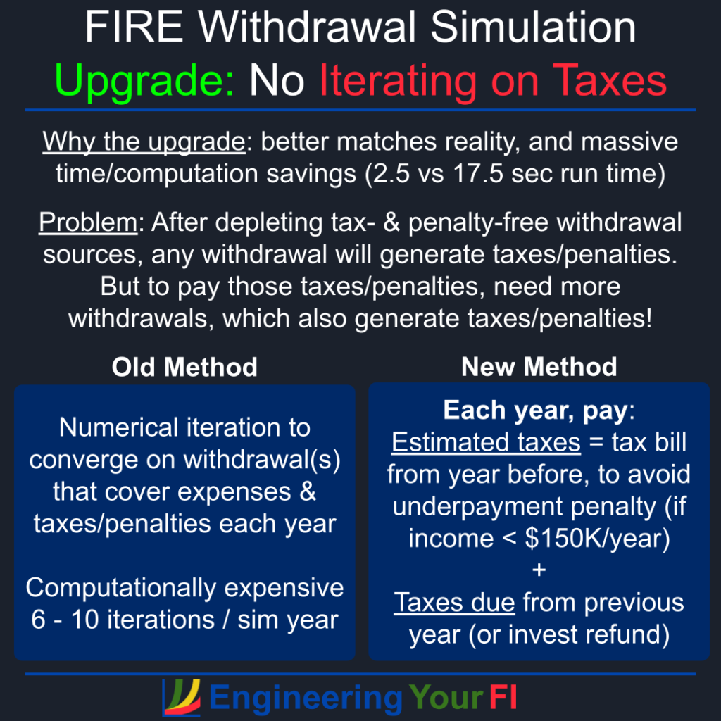
No More Iteration
Something I’ve mentioned in previous posts is that I would need to build an iteration capability for the TPM method, just like I did for the traditional method. Because if all we have left are accounts that generate taxes and/or penalties, we’ll need to iterate to figure out how much more we need to withdraw to pay for those taxes and/or penalties, etc.
However, I could see that this iteration was adding a LOT of time to an already computationally expensive simulation. Six to ten iterations was common, and it had to do that every year of the simulation. Ugh.
Then thinking about it even more, I realized that it’s also not how taxes work in general anyways.
Typically you pay estimated taxes to the IRS throughout the year, either via automatic paycheck/withdrawal withholdings or the four required estimated tax payments (sometimes called quarterly payments, even though they aren’t really aligned to the quarters). Then you settle up with the IRS the following spring when you do your tax return.
New Non-Iteration Method
So I decided to take the same approach in the TPM method, as well as the Traditional method to be consistent.
For each year, first I pay as estimated tax the total tax bill generated the year before, which will avoid an underpayment penalty as long as you make less than $150K/year (otherwise you need to pay 110% of last year’s tax bill to be safe). Then I pay the tax still due from the previous year (or collect the relevant refund and invest it in the post-tax account).
The result: no more convergence necessary! You just have to extract enough cash to pay for that year’s expenses and the above tax amounts – which are both functions of the previous year’s income, not the current year.
This approach is a massive time and computation saver: employing iteration with the TPM method in the scenarios I discuss below, it takes 17.5 seconds to run. Without iteration it takes just 2.5 seconds, and even results in a slightly higher final total.
Here’s a diagram overview:
Example
How does it give a higher total though? Well, this approach can actually SAVE you money if your income consistently goes up over time, as one would expect in general with Social Security Income and then Required Minimum Distributions (RMDs) kicking in and then growing over time (especially with inflation).
Let’s look at an example. Let’s say you retire and need $40K a year for expenses. You manage to use only tax-free sources of money for a number of years, but then you have to start using assets that generate 10% in taxes or penalties when you withdraw.
- Year 1:
- $0 in owed taxes, $0 in estimated taxes (since paid $0 in taxes the year before), total taxes paid = $0
- income generated to pay total taxes and expenses = $40K
- tax bill of $4K
- Year 2:
- $4K in owed taxes, $4K in estimated taxes (previous year’s bill), total taxes paid = $8K
- income generated to pay total taxes and expenses = $48K
- tax bill of $4.8K
- Year 3:
- $0.8K in owed taxes, $4.8K in estimated taxes, total taxes paid = $5.6K
- income generated to pay total taxes and expenses = $45.6K
- tax bill of $4.56K
- Year 4:
- -$0.24K in owed taxes, $4.56K in estimated taxes, total taxes paid = $4.32K
- income generated to pay total taxes and expenses: $44.32K
- tax bill of $4.432K
- Year 5:
- -$0.128K in owed taxes, $4.432K in estimated taxes, total taxes paid = $4.304K
- income generated to pay total taxes and expenses: $44.304K
- tax bill of $4.4304K
You can see how the tax bill is converging on $40K / 0.9 = $44.444K, which is the amount you would pay each year if you were to use iteration to converge on the amount you’d need to withdraw to pay both the 10% penalty on the withdrawal and still have $40K for expenses.
The total taxes paid over those 5 years is $0K+$8K+$5.6K+$4.32K+$4.304K = $22.224K, which is very close to the $4.444K*5 = $22.22K you’d pay if you converged every year.
However, you can see how the non-iteration approach means you PAY LESS IN THE BEGINNING, and converging only after a number of years. The first year you pay $0 in taxes instead of $4.444K, and the first two years you pay $8K in taxes instead of $8.888K.
Essentially you are converging with each passing year instead of paying the final converged amount $4.444K every year. And by paying less in the beginning, your money will have more time to grow, and thus you are likely to end up with more money in the end / less likely to run out of money.
But, again, this assumes your income typically stays the same or grows over time – if it were to drop significantly, you’d face the opposite problem of paying too much taxes for a few years, until it can converge on the lower value.
In general though, regardless of income rising or dropping, you end up paying about the same amount in taxes WITHOUT the expensive iteration needed, so it helps tremendously with this analysis.
Odds and Ends
This new approach for taxes means the user needs to provide their tax bill and how much they paid in taxes for the year before the simulation starts – those values are now vital parts of the tax calculation.
This new approach also means you might owe taxes or be owed a tax refund the year after you die – which, again, is how the world really works. And just like in the real world, your estate will cover it, or it won’t. You’ll be gone, so you don’t have to worry about covering living expenses. And if your estate doesn’t cover a tax bill, your descendants (in general, see exceptions) do NOT have to worry about paying the tax bill.
One final bit of info: as far as I can tell after extensive searching, your estimated tax payments do not need to include estimated penalties. Thus the TPM and Traditional methods always pay any penalties incurred in the subsequent year. Hopefully that’s correct – please let me know if it’s not. If not, I have the infrastructure in place to pay estimated penalties based on the previous year, just as I do with taxes, so that’ll be an easy change to make.
Dividends
Previously I used the user-input values for qualified and non-qualified dividends every year of the simulation. Of course this wasn’t a very accurate model unless your post-tax account stayed around the same balance the entire simulation (in 2022 dollars). But at least it was on the conservative side for scenarios where the post-tax balance grows to larger amounts.
But with highly strenuous scenarios taking the post-tax balance to $0, obviously it makes no sense to keep getting dividends from an empty account. And that error can lead to results that are much better than they should be.
So I modified the user-input values for dividends to be the dividend yield values instead: when multiplied by the post-tax account balance, you obtain the dividend amount.
I know that dividends are computed as a function of how many shares you have, and not the overall account balance, but I decided to simplify the model and use the overall account balance. I’d like to avoid having to track individual share quantities in addition to everything else being tracked, and I suspect this simplified model will be good enough for our purposes. I can add that level of granularity to the simulation tool in the future if needed.
Test Scenarios
Let’s employ a couple scenarios we’ve used before, but with much higher expenses.
Betty’s Filing Status: Single
We’ve discussed Betty before, but now we’re going to ramp up her expenses!
Let’s increase Betty’s expenses from $40K to $67K. Why $67K? Turns out if you increase Betty’s expenses $1K at a time, $67K is the first amount where she runs out of money before age 92 using the TPM method. And I want to compare the TPM and Traditional methods when they both run out of money, to see what age that happens.
And as usual, those expenses (and all other values) are always in 2022 dollars, so nominal expenses will increase (beyond $67K) with inflation.
I’ve also moved the $20K in cash to the Roth account as a contribution, to make comparing scenarios easier, as I did in a previous post.
Finally, I’m now using a qualified dividend yield of 1.6%, based on the 5-year average dividend yield of the total stock market fund VTSAX, and a non-qualified dividend yield of 0%. Thus for a $400K post-tax balance, qualified dividends will equal $6400 (instead of the $10K used previously) and non-qualified dividends will equal $0 (instead of the $100 used previously). I also subtract that dividend yield from the standard historical 7% (after inflation) ROI used to model investment growth for the post-tax (taxable) account – because that historical ROI includes the impact of reinvesting dividends.
For the traditional method, the assets vs time plot is:
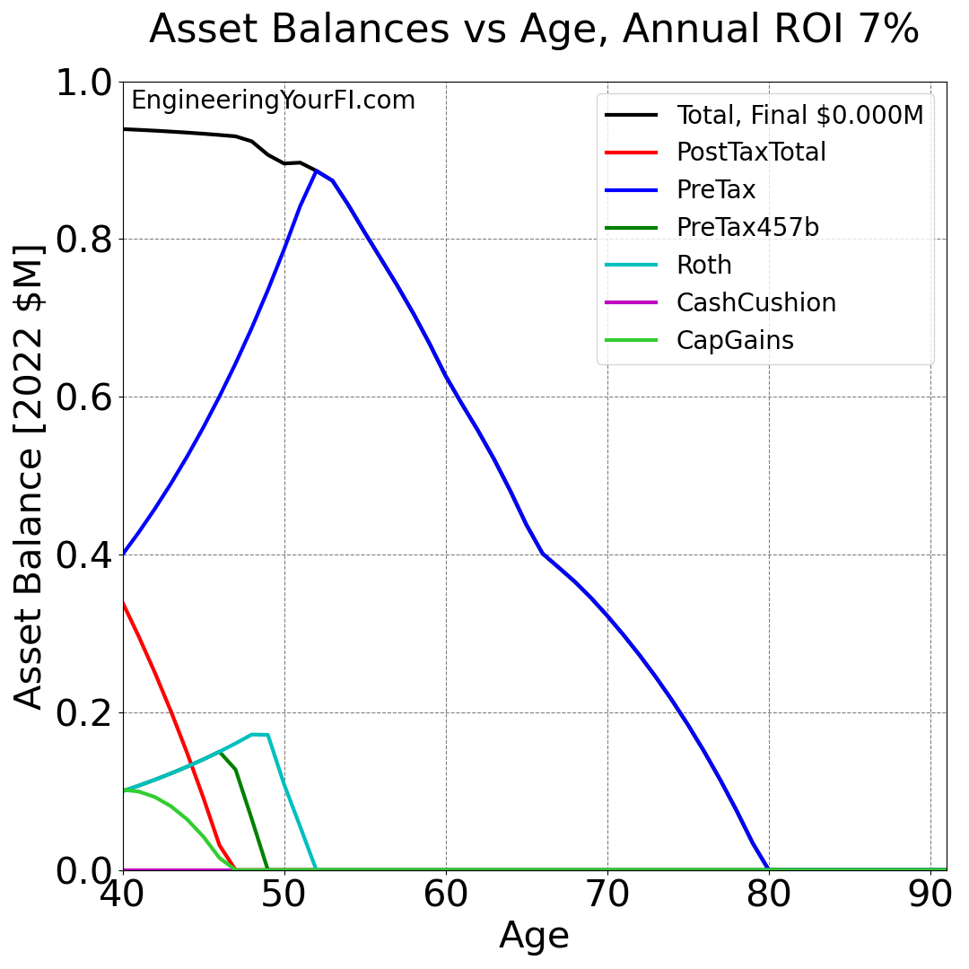
You can see how the PostTax balance goes to zero first, then the 457b balance, then the Roth balance, all by the time the sim hits age 52. At that point, the PreTax account is all that’s left (matching the total balance) and that runs out of money about 28 years later at age 80.
Now let’s run the same scenario with the TPM method:
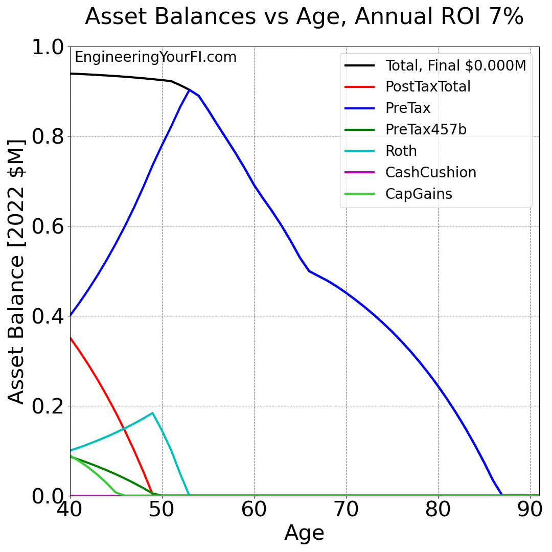
Now Betty runs out of money at age 87 instead of 80 – the TPM method bought her seven more years!

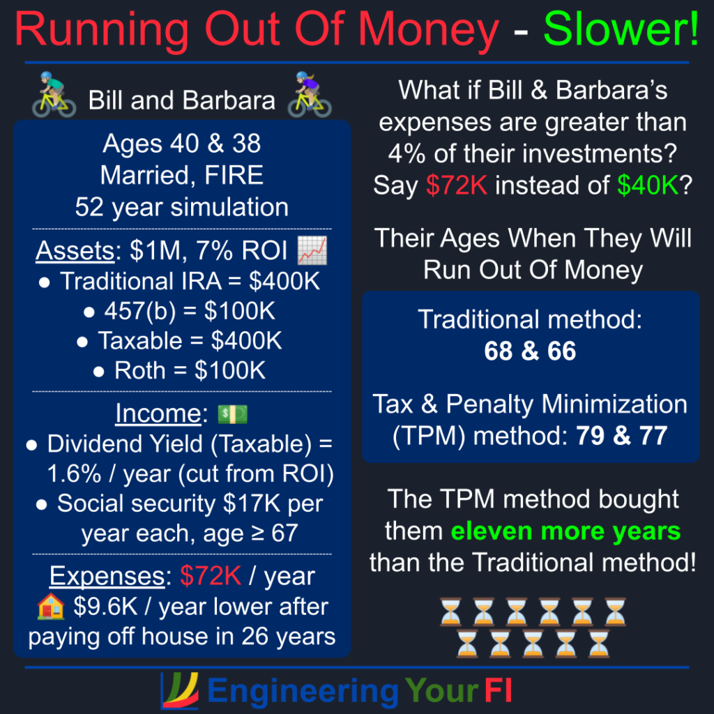
Bill and Barbara’s Filing Status: Married Filing Jointly
In the same previous post where we met Betty, we also met the married couple Bill and Barbara. Just like for Betty, we’ve moved the $20K cash to the Roth account, and we’re using a qualified dividend yield of 1.6% and a non-qualified dividend yield of 0%.
For Bill and Barbara, increasing their expenses $1K at a time leads to running out of money with the TPM method for the first time at $72K. So let’s use that for expenses in both methods.
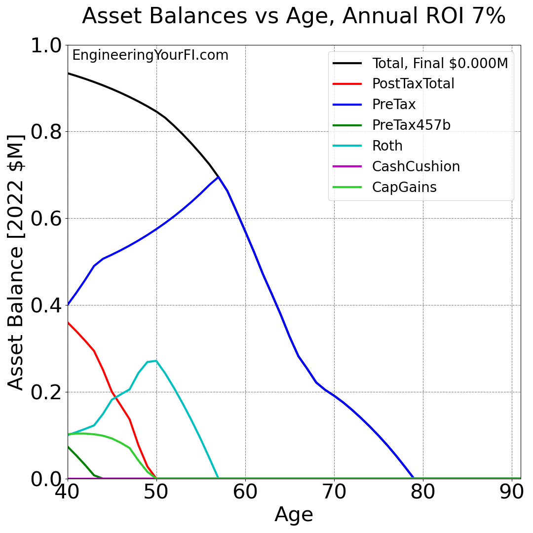
For the traditional method, the assets vs time plot is:
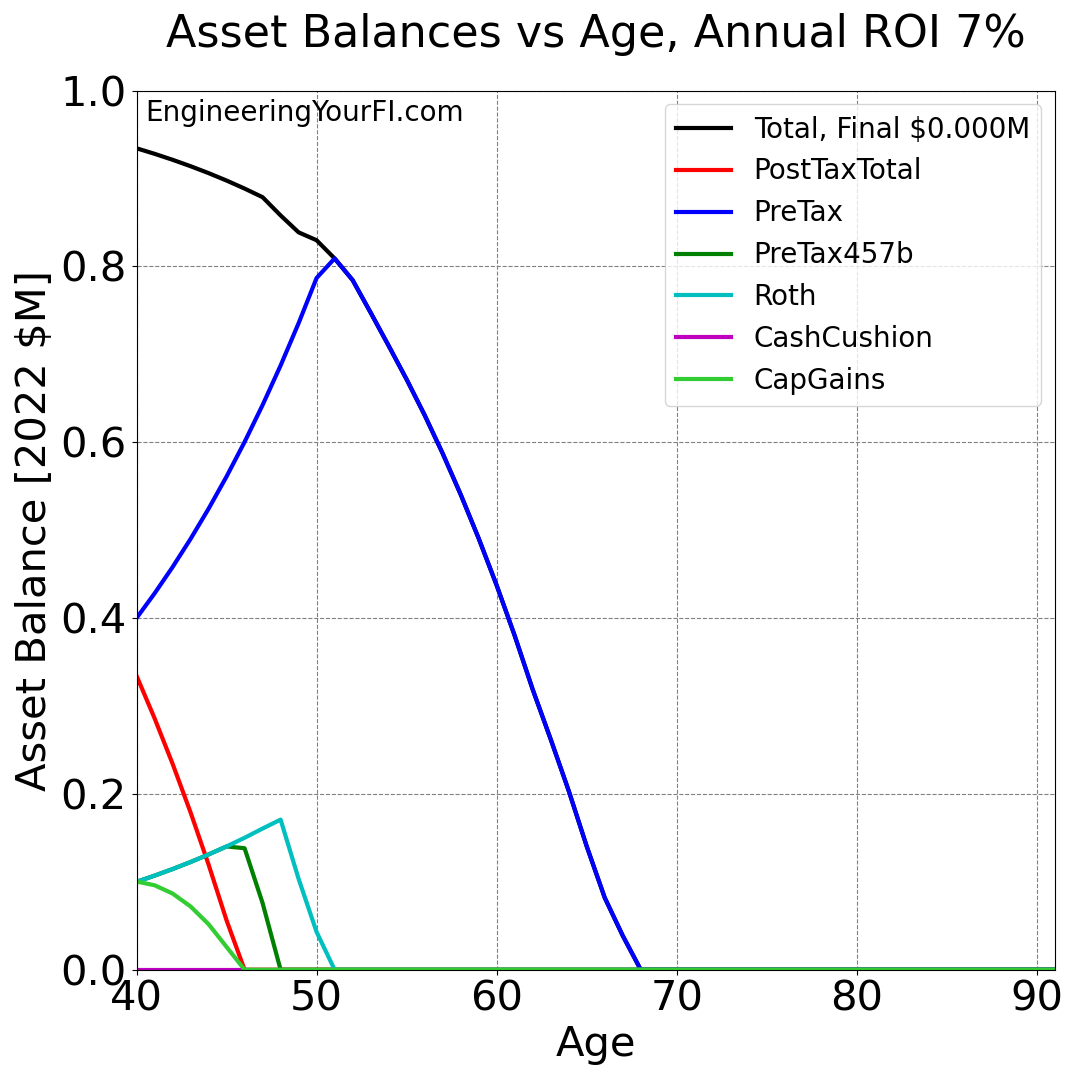
Bill and Barbara run out of money at age 68 (for Bill, Barbara is 66) – not too bad for such an aggressive expense level. But it’s still well before the average age of death (76) in the United States in 2021.
Now let’s run the TPM method for Bill and Barbara:
Bill and Barbara now run out of money at age 79 and 77 – gaining 11 years of financial solvency by using the TPM method instead of the traditional withdrawal method!
The TPM method gets Bill and Barbara to their late 60’s with a much higher balance than the traditional method, so that when their expenses drop (mortgage paid off) and their income increases (social security kicking in at age 67), it’s able to hobble along much further before running out of money.
Now we probably could have made the traditional method last a bit longer if we had started social security earlier than the full retirement age of 67, but I wanted to stick to a standard scenario as much as possible.
And also of course remember that I’m just using the average historical after-inflation market return of 7% each year – in reality the returns will be highly variable each year, but over time they will likely match this historical long term return rate.
Future Work
Stress Testing Analysis
Now that the TPM method is capable of going down to $0, I can finally do the analysis I’ve been aiming for over the last month – very exciting!
My initial plan is to look at a range of expense and ROI levels versus final asset balance or when the money runs out, for both the traditional and TPM methods. I want to see how each method does on its own, and how they compare.
Hopefully that’ll happen this next week somehow, but my son and daughter are both home from school all next week for the holidays, so I’m not sure how much time I’ll have to work on it. But I’ll give it the ol’ college try!
I will also provide all the updated code when I get that analysis done and posted.
Other Ideas
Any time I do any development or analysis, I usually come up with lots more future work ideas. This development has been no exception. Here are some of the top ideas:
- Right now if the TPM reaches the point of employing the numerical integration subroutine to obtain the needed cash with minimal taxes/penalties, it always starts from the current totals for standard income and LT cap gains. However, if we could reduce the standard income such that we can sell more post-tax lots and stay within the 0% LT cap gains bracket, that could potentially provide more cash with zero additional taxes (since LT cap gains are a fraction of the cash you would receive when selling, vs 100% of the pre-tax account withdrawals counting as standard income). We can employ a similar numerical integration method for this approach as well, taking finite steps until reaching an optimal amount of standard vs LT cap gain income.
- I read on nerdwallet that while you don’t have to pay the 10% penalty for early retirement account withdrawal until you file your tax return in the spring, generally the IRS requires a 20% withholding for any early withdrawals for taxes. I’d like to add that to the TPM numerical integration model to see what kind of impact it has.
- Save/capture the taxes and penalties for each step in the TPM Numerical Integration method for visualization and understanding of how those values evolve for each year the numerical integration is employed.
- Identify the code that takes most of the computation in the TPM Numerical Integration method, likely via a python profiler tool, and employ a tool like Numba that can convert those slowest chunks into much faster compiled code. That could potentially greatly speed up the method, and allow for smaller steps that produce a more optimal answer. But it might also not speed up the code that much, and thus not really be worth the effort. Especially if it takes only 2.5 seconds to run the full simulation and get an final answer that’s optimal within $100.
Conclusions
The main takeaways from this week’s work:
- The TPM numerical integration seems to work pretty well, and a $100 step seems to be a nice balance between speed and accuracy.
- I’ve dropped the effort to iterate on withdrawals for tax and penalty payments each year, replacing it with an approach using previous year tax values that better matches how we actually pay taxes and dramatically reduces required computation.
- I’ve changed constant dividend inputs provided by the user to dividend yield inputs provided by the user, so that dividends are a function of the yield values and the post-tax account balance (and I recognize this is an approximation, since dividends are typically computed using number of shares owned instead of account balance).
- For a couple of reasonable early retirement scenarios I tried, filing single and married filing jointly, the TPM makes your money last years longer.